Introduction to Formulas

This article will focus on covering a few basic formulas and we will move on to complex formula in later articles.

To enter a formula in excel:
Select the cell where you want the result of the formula to be displayed.
In the field for ‘fx’, enter the formula.

Press ‘Enter’. Now, you will see the result in the selected cell.

If there is any error in the formula entered by you, you will get an alert about the error and also a suggestion for a possible correction.
We will cover the below kinds of formula. There can also be different combinations of these kinds. Also one thing to remember is that you can accomplish the same task in Excel through different ways.

Simple formula:
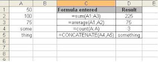
These are the simplest of formula and can be used to calculate the results of simple mathematical calculations. Below are a few examples.
As you can see in the fourth example, there can be nested formula as well.

Formula with references:
This kind of functions is used when one or more values used in your calculation are derived from the value of another cell in the sheet.

Functions:
Excel provides a whole lot of built-in functions that can be readily used. Below, you can see some of them. I would not cover each and every function here, but in the future topics, I will show how to use these functions to solve some common problems.

Validating Data in a Sheet

To avoid having incorrect data in your sheets, you can define some validations on the data you have. Whenever these values are modified or a new data is entered, the validation would be performed. This allows you to keep a check on users entering invalid data.

To use any of the excel provided validations of your data, use the option Data --> Validation…

Suppose, you are making a list of things to carry on your next adventure trip which looks something like the one shown below:
Now, you want to have a validation that the field ‘Quantity’ can only contain whole numbers, Select the cell range where you want to apply this validation and click on Data --> Validation… Now, in the Validation Criteria in the ‘Settings tab’, choose ‘Whole Number’ for Allow, If you want to have more validation like quantity should be in a range or greater than some value, etc, you can select it appropriately.
In the ‘Input Message’ tab, you can enter any message that you want to show to the user when he/she selects the cell for which the validation is being applied.
If you want to show a message to the user when he/she enters a value in the cell which does not satisfy the validation criteria provided by you, then provide the appropriate message in the ‘Error Alert’ tab. This message could either stop the user from entering an invalid data or show it as a warning or information message,
Click on any of the cells on which you have applied the validation and you will see the input message.
Enter an invalid data and you will see the warning message.

Filter and Sort Columns

Filtering and Sorting based on a particular column’s values are the most commonly used features in Excel. Continuing with the same workbook used by me in some previous examples (shown below), we can see various ways in which this sheet can be filtered.The most commonly used option for filtering and sorting columns is by using the Auto Filter. Select all the columns that you may need to filter your data on (here I choose Age and Gender) and then choose the option Data --> Filter --> AutoFilter.

Now, you have the filter option available on the required columns. Click on the drop down arrow and choose the required data based on which you want to filter. For example, I would be interested in the females in the list and hence, I would choose Females in the drop. The filtered result would look like this:

Now, I want to sort them on the ascending order of age. So, I would first remove the filter that I have applied on the Gender column and then choose ‘Sort Ascending’ in the Age filter. The result would look like this:

To remove a filter, just to choose (All) in the filter. It will show all the results.

If you want just the users who are between 30 and 40 years of age, select (Custom..) from the filter drop down and in the new window, provide the filter criteria. Another way of sorting data is by using the Sort option. Select all the columns in the sheet and then choose Data --> Sort…

In the resultant window, provide your sort criteria. Here, I am sorting the users by the first name first and then their gender and then their age.In this way, you can choose different filter criteria based on your needs.

Split text into different columns

This is another simple yet very helpful feature in Excel. This allows you to split your data in one column into multiple columns based on a simple condition.

The condition could be:
- A delimiting character
- A fixed length of text

Consider an example where you have user information in your excel with the data separated by semi-colon.

In order to get this data aligned properly in different columns, select all the data in the first column and use the option Data --> Text to Columns..
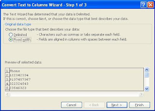
Select the ‘Delimited’ option for Original data type.
Select ‘Semicolon’ as the delimiter to be used. In bottom ‘Data preview’ pane, you will be able to see the preview of how your sheet would look like after applying the condition.
In the next screen, you can set the data format for each column. Then click on the ‘Finish’ button.
The data would now have been adjusted into different columns.

Now, if you want the Name column to be split into two columns, one containing the first name and the other, the last name:

Insert a new column between the Name and City columns and follow exactly the same procedure for the first column but this time selecting ‘Space’ as the delimiter.

Now, if you want the phone number to be split into the country code (first two digits) and the actual phone number, you may again use the ‘Text to Columns...’ feature.

This time, select column G and choose ‘Fixed width’ for the ‘Original data type’.
In the scale to measure character length, set the delimitation for 2 characters.
Once you have finished formatting your sheet, you may need to correct your columns headings:

Protect your files

Excel offers various options to protect sensitive information from others. Today, we discuss ways to restrict users from reading or writing to a excel document.

Open your excel file that you want to protect and go to Tools --> Options. Select the 'Security' tab.

If you want only authorized people to be able to open your workbook, then set a password in the text box for ‘Password to open’. (You can also choose any encryption type for your password by clicking on the ‘Advanced’ button)

If you want only authorized users to be able to modify your workbook, then set a password in the text box for ‘Password to modify’.

You can use any or both of these password settings based on your requirements.

Transpose the Matrix

One simple yet useful feature in Excel is to transpose the selected cell range in the sheet.

Assuming you have a matrix/table like the one shown below and you want to interchange its rows and columns, here are two ways how you can achieve it.

Using Paste Special:
Copy the range of cells you want to transpose (in our case A1 to F4) and then right click on the cell where you want to have the transposed matrix (in our case A7). Select ‘Paste Special’ from the options.

Tick the ‘transpose’ option in the Paste Special menu and click on OK.

Using TRANSPOSE Operation:
Select the range of cells where you want your transposed matrix (in our case A15 to D19) and enter the array operation in the fx tab:
=transpose(A1:F4) and press CTRL+SHIFT+ENTER

Advantage of using Paste Special is that you can copy the format and the formulae of the copied cells along with the cell values, which is not possible using the array operation of TRANSPOSE. The advantage of the array operation is that when you modify the parent matrix, automatically the child matrix is also updated. So, you can use any of the two options based on your requirement.

Freeze those panes!!!

Excel provides a useful feature of freezing or locking a particular pane in a worksheet while you can scroll through the remaining contents in the sheet. This feature is quite useful when you have a lot of rows or columns in your sheet and you need to often scroll through the sheet to view them. This feature improves the readability of the document.

Freeze top pane:
Suppose you have a long list of names and with the column headers in the first row, then you would prefer to keep the first row static while scrolling through the list of names.

To freeze the top row, just click on the cell A2 in the sheet and use the option Window-->Freeze Panes.

Now, you will notice that even when you scroll down, the column headers remain static.
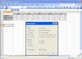
Freeze left pane:
If you want the first column in the sheet to be static/frozen, you can click on the cell B1 and then freeze the panes.

Freeze top and left panes:
If you want both the top and the left panes to be frozen, simply use the option on the cell B2. You will be able to scroll horizontally and vertically through your sheet keeping the first row and first column immovable.
The idea is you should always select the first movable cell when you select the ‘Freeze Panes’ option.

To unfreeze the panes, use the option Window-->Unfreeze Panes.

Getting Started

Hello Everybody,

Greetings from Roshan!

Here, I will share useful tips that can simplify your work in Excel and make working with Excel a pleasure. Instead of wasting a lot of time in searching for relevant information, just connect to my blog and look-up what you need. I assure you will find most of the important topics in here in a few days.

Please feel free to share your feedback on the quality of articles and suggestions for improvement. Also, let me know if there any topics you need information on and I can post them for you.

Regards,
Roshan