Transpose the Matrix

One simple yet useful feature in Excel is to transpose the selected cell range in the sheet.

Assuming you have a matrix/table like the one shown below and you want to interchange its rows and columns, here are two ways how you can achieve it.

Using Paste Special:
Copy the range of cells you want to transpose (in our case A1 to F4) and then right click on the cell where you want to have the transposed matrix (in our case A7). Select ‘Paste Special’ from the options.

Tick the ‘transpose’ option in the Paste Special menu and click on OK.

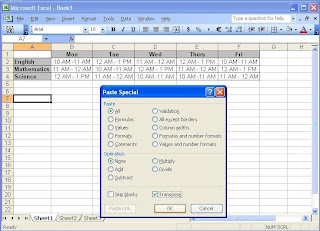
Using TRANSPOSE Operation:
Select the range of cells where you want your transposed matrix (in our case A15 to D19) and enter the array operation in the fx tab:
=transpose(A1:F4) and press CTRL+SHIFT+ENTER

Advantage of using Paste Special is that you can copy the format and the formulae of the copied cells along with the cell values, which is not possible using the array operation of TRANSPOSE. The advantage of the array operation is that when you modify the parent matrix, automatically the child matrix is also updated. So, you can use any of the two options based on your requirement.

Freeze those panes!!!

Excel provides a useful feature of freezing or locking a particular pane in a worksheet while you can scroll through the remaining contents in the sheet. This feature is quite useful when you have a lot of rows or columns in your sheet and you need to often scroll through the sheet to view them. This feature improves the readability of the document.

Freeze top pane:
Suppose you have a long list of names and with the column headers in the first row, then you would prefer to keep the first row static while scrolling through the list of names.

To freeze the top row, just click on the cell A2 in the sheet and use the option Window-->Freeze Panes.

Now, you will notice that even when you scroll down, the column headers remain static.
Freeze left pane:
If you want the first column in the sheet to be static/frozen, you can click on the cell B1 and then freeze the panes.

Freeze top and left panes:
If you want both the top and the left panes to be frozen, simply use the option on the cell B2. You will be able to scroll horizontally and vertically through your sheet keeping the first row and first column immovable.
The idea is you should always select the first movable cell when you select the ‘Freeze Panes’ option.

To unfreeze the panes, use the option Window-->Unfreeze Panes.

Getting Started

Hello Everybody,

Greetings from Roshan!

Here, I will share useful tips that can simplify your work in Excel and make working with Excel a pleasure. Instead of wasting a lot of time in searching for relevant information, just connect to my blog and look-up what you need. I assure you will find most of the important topics in here in a few days.

Please feel free to share your feedback on the quality of articles and suggestions for improvement. Also, let me know if there any topics you need information on and I can post them for you.

Regards,
Roshan